Since ever, one had to choose between efficient models and explainable models. On one side, simple models like logistic regression are interpretable but lag on performances. On the other side complex models like Boosted Trees or Neural Network reach incredible accuracy but are hardly understandable.
Since 2012, researchers from Microsoft studied and implemented an algorithm that breaks the rules: Explainable Boosting Machines (EBM). EBM is the only algorithm that gets free of this performances vs explainability ratio curve.
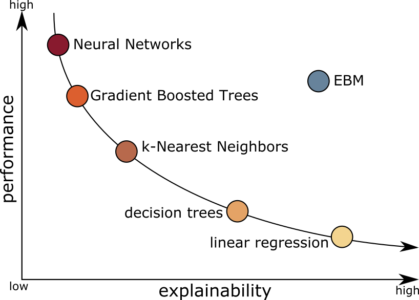
With EBM you do not have to sacrifice performances when explainability is a requirement, and you have explanations for free with top performances. One important aspect of EBM is that it is naturally interpretable. We do not talk about explaining complex models with methods like Lime, Shap, or GramCam: EBMs are explainable by nature. One can directly see how the model uses each feature. For example, see this plot of the global explanation for one variable:
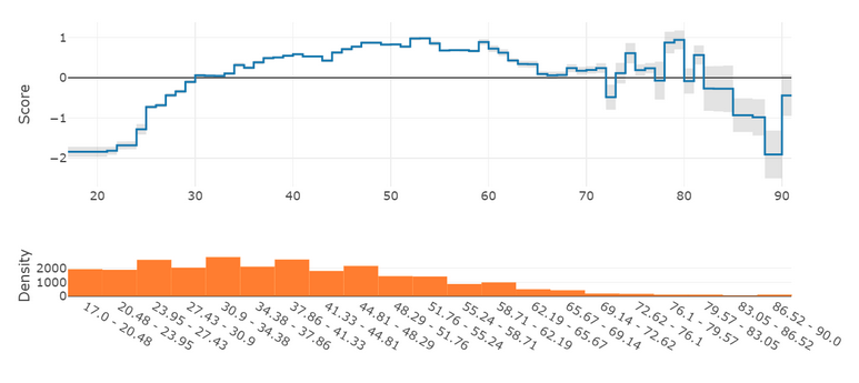
The blue line is how the model uses the feature, not an estimation. These graphs are invaluable to understand the inner working of a model. They are also of great help to debug: If the model overfits a feature somewhere, you see it immediately (do you see the overfit here?). These are the kinds of issues that are hard to spot with Lime or Shap. One can argue that this is the aim of the data exploration phase. Unfortunately, it is so easy to miss something during this stage that it is nice to - somehow - rely on the model itself.
So how does EBM work? Does this seem too good to be true?
We will see that this is possible thanks to a clever combination of several techniques.
Generalized Additive Models
Let's start with the foundation that makes EBM explainable. EBM is a type of Generalized Additive Model (GAM), formalized by Trevor Hastie and Robert Tibshirani. The full description of this family of models is available in chapter 9 of their book Elements Of Statistical Learning. A GAM is any model that satisfies this formula:

The f functions are named shape functions. The g function is the link function. You probably noticed that this is very similar to linear regression:

And you are right! Linear regressions are also GAMs where:
- The shape functions are multiplications (with the weights).
- The link function is the identity.
Similarly, logistic regression is also a GAM where the link function is the logit.
The mathematical definition of GAMs defines why they are explainable: Plot the shape functions and see how the model uses each feature. It's that simple. The plot of the previous section is just that: A plot of a shape function.
Better Than GAM: GA²M
So GAMs are explainable by design. However, they have one significant drawback: They use each feature individually, missing any relation between the two of them. Even a single decision tree combines features to make its predictions. Note that in my experience, this simple approach gives very decent performances.
EBM brings the first improvement to GAMs by also using pairs of features on the additive terms:

Such models are called GA²M: Generalized Models with Interactions (no, there is no error in the definition. Finding a name for an algorithm is not always easy).
The point is that shape functions that use two features are still explainable: Instead of being rendered as lines, curves, or steps, they are displayed as heatmaps. Sure they are harder to interpret, but they are. On the other way, this allows to combine several features and boost performances.
Before we continue on the improvements of EBM over GAMs, let's see how to make a prediction.
EBM Inference
Another advantage of EBM is that its inference is light in terms of computation. That's a point in production environments where the prediction latency must be as small as possible.
The following figure shows all steps of a prediction:
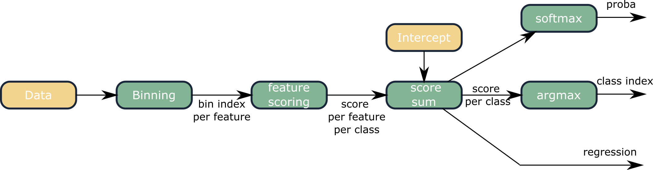
The computation-intensive parts are the bins lookup and the addition!
The first step consists of discretization for continuous variables, and mapping for categorical variables. Continuous variables are split into bins. During the binning step, the features are mapped to an index value. Each index is then associated with a score. This is done for each feature. Ultimately, the prediction is the addition of all scores plus an intercept/bias. For multi-class classification, there is one score per class. Depending on the task, post-processing may be used (the link function):
- For regression, the sum is directly the predicted value.
- For classification, the class with the maximum score is the predicted class.
- For class probabilities, a softmax is applied to the score of each class
Let's follow these steps with an example. The following figure highlights the prediction of the first row of a dataset with a model using two features:
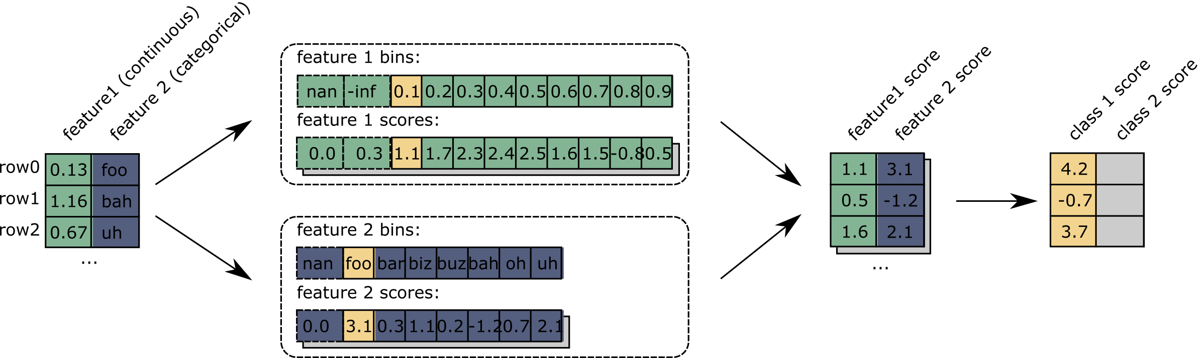
These steps are all expected on a GAM. However, the initial binning and scoring parts are more intriguing: They are the shape functions but are independent of any algorithm or formula. They could represent any shape function: a spline, a decision tree, or even a neural network.
Let's see where this discretization comes from.
Fitting The Shape functions
The EBM training part uses a combination of boosted trees and bagging. A good definition would probably be bagged boosted bagged shallow trees. The core of the algorithm uses boosted trees, as shown in the following figure:

Shallow trees are trained in a boosted way. These are tiny trees (with a maximum of 3 leaves by default). Also, the boosting process is specific: Each tree is trained on only one feature. During each boosting round, trees are trained for each feature one after another. It ensures that:
- The model is additive.
- Each shape function uses only one feature.
This is the base of the algorithm, but other techniques further improve the performances:
- Bagging, on top of this base estimator.
- Optional bagging, for each boosting step. It is disabled by default because it increases the training time a lot.
- Pairwise interactions.
Depending on the task, The third technique can dramatically boost performances: Once a model is trained with individual features, a second pass is done (using the same training procedure), but with pairs of features. The pairs selection uses a dedicated algorithm that avoids trying all possible combinations (which would be infeasible when there are many features).
Finally, after all these steps, we have a tree ensemble. These trees are discretized, simply by running them with all the possible values of the input features. This is easy since all features are discretized. So the maximum number of values to predict is the number of bins for each feature. In the end, these thousands of trees are simplified to binning and scoring vectors for each feature.
So these vectors are the results of thousands of trees that exist only for a few minutes. As soon as we built them, we do not need them anymore!
Conclusion
The times when one had to choose between accuracy and explainability are over. EBMs can be as performant as boosted trees while being as explainable as logistic regression.
EBMs belong to the family of GAMs - Generalized Additive Models -. They use boosted trees encoded in a way that allows simple inference and explanations.
EBMs are part of the InterpretML project from Microsoft. I encourage any data scientist working on tabular data to try it. We achieved performances on par with XGBoost on several tasks, while clearly understanding how the model uses each feature. If you work in a domain where explainability is mandatory, or runtime performance is key, you should give it a try.